Hooke’s Law and the Simple Harmonic Motion of a Spring

 

Purpose:  To determine the force constant of a spring and to study the motion of a spring and mass when vibrating under influence of gravity.

Equipment: Spring, masses, weight hanger, meter stick, support stand with clamps,  motion  detector, LabPro interface, wire basket.
Introduction: When a spring is stretched a distance x from its equilibrium position, it will exert a restoring force directly proportional to this distance. We write this restoring force, F, as:
                        1)  F  =  -kx       
where k is the spring constant and depends on the stiffness of the spring.  The minus
sign remind us that the direction of the force is opposite to the displacement. 
Equation 1 is valid for most springs and is called Hooke’s Law.

If a mass is attached to a spring that is hung vertically, and the mass is pulled down
and released, the spring and the mass will oscillate about the original point of
equilibrium. Using Newton’s second law and some calculus we can show that the
motion is periodic (repeats itself over and over) and has period, T (in sec), given by 

2)  T  = Square root of 4pie^2/k (m) 

    
where m is the mass supported by the spring.

Procedure: We began by hanging a spring on to a rod and measuring the positon of the lowe end of the spring.  We then placed a 350 gm mass on the spring and observe its positon. Then we continued to do this for masses of 450, 550, 650, 750, 850, 950, 1050, recording how far the spring stretched for each mass.  The results were as follows;

Y- axis     X - axis                                           Using equation 1 F= - kx
no wight     0 displacement                                       we got 2.35 kg = K
350             15 cm
450             19 cm                                                            converting to newtons  23.5 N
550             23.5 cm
650              28 cm
750              32.5 cm
850              36.25cm
950              41 cm
1050            44.5 cm

We then turned on the logger pro and began to collect data on a positon vs time graph.  We hanged each mass and stretched it 10 cm. WE release the masss and abserved teh subsequent motin.  We allowed for 5 cycles and calculated teh period of motion.  Repeating this steps we were able to create a data table which gave us average T and m values.  Using tyhe data for the last trial with

                    M =  1050 g
we fited the data to a sinusoidal function using the analyze/ Curve Fit option.  From this we were able to determine the period of the amplitude. 



Conclusion:  We had trouble with our units.  For some reason when we plug in our numbers in to equation two we got a number that was way off.  So we couldnt tell if we had goten the first equation wrong which seems almost imposible because its just the force (weight) x the displacement ( strech).  So when we compared our k value in part 1 with the one in part two we got a 15 unit difference.

The Ballistic Pendulum

Purpose:  To use the ballistic pendulum to determine the initial velocity of a projectile using conservation of momentum and conservation of energy.
Equipment: Ballistic pendulum, carbon paper, meter stick, clamp, box, triple beam balance, plumb. 
Introduction: In this experiment a steel ball will be shot into the bob of a pendulum and the height, h, to which the pendulum bob moves, as shown in Figure 1, will determine the initial velocity, V, of the bob after it receives the moving ball.  If we equate the kinetic energy of the bob and ball at the bottom to the potential energy of the bob and ball at the height, h, that they are raised to, we get:
      

( K.E ) bottom = ( P.E)top

      ½ ( M + m ) V² = ( M + m ) g.h

 where M is the mass of the pendulum and m is the mass of the ball. Solving for V we get:

        V  = √ 2gh            …………….                                                                                                   

(1) Using conservation of momentum we know the momentum before impact (collision) should be the same as the momentum after impact. Therefore:

Pi= Pf

      or

           mv0 = ( M + m) V 

(2) where v0 is the initial velocity of the ball before impact. By using equations (1) and (2) we can therefore find the initial velocity, v0, of the ball. We can also determine the initial velocity of the ball by shooting the ball as above but this time allowing the ball to miss the pendulum bob and travel horizontally under the influence of gravity. In this case we simply have a projectile problem
where we can measure the distance traveled horizontally and vertically (see Figure 2) and then determine the initial velocity, v0, of the ball.

M + m Starting with equations:
    ∆x = voxt + ½axt² 
    (3) ∆y = voyt + ½ayt

 ( 4 )
You should be able to derive the initial velocity of the ball in the horizontal direction (assuming that
∆x and ∆y are known). Include this derivation in your lab report.

We set up our ballistic pendulum loade the triger with the ball and shoot it two times.  From this we got a average hight (h).  Then we toke the pendulum and the ball and got their masses.  Using equations 1 and 2  we were able to determine our initial velocity. 

 

Next we went on to determen initial velocity from range and fall. We placed the pendulum up on the rack so that it wouldnt interfere with balls motion. We clamped the frame to the table so that it wouldnt move and placed a piece of carbon paper on the floor. We shoot the ball a few times and took our average positon to be delta X.  From delta X and delta Y(the hight) we used equation 3 to solve for initial velocity. Having the two velocities we toke a percent diffrence and agreed that the free fall experiment was the more accurate one since there is no interaction with any objects and we toke the average distance of the fall which were almos identical.  We trust the conservation of momentum as well but fell that there could be more room for error since we got diffrent heights almost every time we fired the ball into the pendulum.

Conclusion:     I learned that through the conservation of Energy we can find a initial velocity as long as we are able to get a hight H Since 1/2 ( M + m) V^2 = ( M + m) g *h .  It was also nice to be able to test our regular kinematics to solve for a free fall initial velocity since it was the basis we started with.  Sources of error could be found in the measurments of either the height or the distance for the free fall.  As for the conservation of energy we found that everytime we shoot the ball into the ballistic we would get a diffent reading.  This could be a big source of error since it lacked consistency.  This is why we agreed that the free fall was probably the more accurate testing out of the two.  After all it did land almost in the same exact location every time we shot it. 

 

Balanced Torques and Center of Gravity

Purpose:  To investigate the conditions for rotational equilibrium of a rigid bar and to determine the   center of gravity of a system of masses.

Equipment: Meter stick, meter stick clamps (knife edge clamp), balance support, mass set, weight hangers,
unknown masses, balance.

Introduction: The condition for rotational equilibrium is that the net torque on an object about some point in the body, O, is zero. Remember that the torque is defined as the force times the lever arm of the force with respect to the chosen point O. The lever arm is the perpendicular distance from O to the line of action of the force.   

We began our experiment by balancing our meter stick in the knife edge clamp.  The meter stick balanced at .496m   Thats .004 short of half the stick

Second we got two different of 100g plus and suspende one on each side of the meter stick at diffrent distances.  We adjusted the positions so the systeem was balance. We ended up with
                mass A of 171.4g @ .285m from 0
                mass B of 121.3 g @ .404m from 0
The masses of the clamps must be included in the calculations because they are part of the mass that affects the balance of the system.

                                       Torque(T) = Force x lever arm
                                    Force is mass a of gravity /  Lever = distance from 0
                                               Tnet = Ta -Tb = 0

(0.1714kg)(9.8m/s^2090.285m) - (0.1213kg)(9.8m/s^2)(0.404m) = 0

0.478720-0.480251= 0.001531

As we can see this number is not quite 0

% diffrence = (theoretical -experimental/ theoretical) x 100

% diffrence is (0.285911m - 0.285 m/ (0.285911m) x 100 = 0.32 %

Third we got the same two masses used above and placed them at different locations on the same side of the support and balance the system with a third mass on the opposite side.  Our three masses where

               mass A of 171.4g @ .200m form 0

               mass B of  121.3 @ 0.300m form 0

              mass C of  272.3 @ 0.261m form 0

 

                                           Tnet = Ta + Tb - Tc = 0

0.335944 +0.356622 -0.696489 = -0.003923

as we can see agin our number doesnt add up to 0

% difference = (0.259530 - 0.261/ 0.259530) x 100 = 0.57 % 

 

   

Next we replaced one of the above masses with an unknown mass.  Readjusting the position of the masses we were able to achieve equilibrium at

                Mass A 171.4 @ .0200m from 0

                mass B  121.3 @ 0.300m form 0

              mas unknown @ 0.419m for 0

 

                                               T net = Ta+ Tb - Tu = 0

     0.335944+0.356622) + mass U kg x 4.106 m/s ^2 = 0.168663 kg - Clamp = 0.146363 kg

 

Unknown mass wighed at 0.1469kg using the balance

That gives a pecent diffrence of .37 %

 

For our next experiment we placed 200 grams at 90 cm mark on the meter stick and balance the system getting a new center of balance.  From this info we calculated the mass of the meter stick 

    position of new 0 on meter stick = .762m

    position previous 0 on metestick = .496m

    Distance of the 200g mass from the new 0 = 0.138m

    Distance of the previous 0 to thenew 0 = 0.266m

 

Tnet=T 200 - Tr = 0

     Calculated mass of ruler 0.103759kg

Ruler weighted @ 0.1032 kg using the balance

% difference = .54 %

 

It is not necessary to include the mass of the clamp holding the ruler in the calculations because it is at the fulcrum, it doesn't affect the balance.

 

Last we imagined that we positojn an additonal 100g mass at the 30 cm mark on teh meter stick.  Calculating the positon of the center of gravity of this combo gave us

 

          T100+ Tr = T 200

Tr = 0.200kg

0 new = 0.261187 kg / 0.4032 kg = 0.647785m

@ experiment its 0.646m

% diffrence = (0.646-0.647785)/ (0.646) x 100 = .28 %

 

Conclusion: This lab was one with the least percent error.  In all of our calculations we were getting less an 1 percent.  We all agreed that there is little room for error in this lab since it wont take much for the ruler to tip to a side. But yet there were some % error. This was probably do to the fact that at times the ruler wouldn't balance stright.  It would rest at a slight angle. We also talked about the inconsestency of the wood being a factor for % error but over all we able to get some very good results with this lab. I cant imagine doing a lab like this with out the use of our new friend, Torque.  Thanks to our torque formulas we were able to investige the conditons for rotational equilibrium of a rigid bar and determine the center of gravity of a system of masses.   

 

 

 





Human Power

Purpose: To determine the power output of a person

Equipment: two meter metersticks, stopwatch, kilogram bathroom scale

Introduction:    Power is defined to be the rate at which work is done or equivalently, the rate at which energy is converted from one form to another.  In this experiment you will do some work
by climbing from the first floor of the science building to the second floor.  By measuring the vertical height climbed and knowing your mass, the change in your gravitational 
potential energy can be found:

∆ PE = mgh

Where m is the mass, g the acceleration of gravity, and h is the vertical height gained. 
Your power output can be determined by 
                   
                        Power  = ∆ PE/∆t,     where ∆t is the time to climb the vertical height h.

We began by taking our weight on a kilogram bathroom scale.  My mass was 77.11 kg
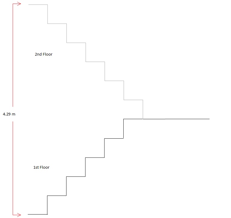
Next the vetical distance between the ground floor and the second floor of the science building was taken.

height = 4.29 m

 

A record keeper and a timer were assigned and at the command of the timing person we ran up the stairs.  Then we did it again for a second trial.  I returned to class and calculated my personal power output in watts using the data collected from each of my climbing trips up the stairs.   Then I got the two trials and obtainthe average power.  When everybody was done we recorded all of our trials as a class and got the average power.  Then i converted my average power output in to units of horsepower.   

 

 

Questions: Is it okay to use your hands and arms on the handrailing to assist you in your climb up the stairs?  Explain why or why not.  Yes its ok because its part of your body and its the strenght of your weight thats making the climb not just your the weight of your legs. 

 

Discuss some of the problems with the accuracy of this experiment.  The measurement of the total hight could have been a little of for we had to use a ruler to do some measurements and then use trig to solve for our hights.  Then there was the person who was incharge of the timer, the reaction time when he said "go" to the actual time we toke off.  To when we ran by him and he stoped the watch.  Those are all factors that could leave room for error. 

 

Conclusion:  Personally I felt that my times and my results of power and horse power were more on the accuarate side than a lot of the class.  In my prespective the faster you ran up the stairs the more power you are using so walking up the stairs doesnt really show how much power you got.   It shows the power that you used to get there but not the max power you have.  Since a lot of the people in class were walking up the stairs I dont believe the class average was a fair average to the amount of power we hold as a classs.  Although it was fun to get a little work out in conveting energy.   

 

   

Centripetal Force

Centripetal Force

 

 

 

Purpose: To verify Newton's second law of motion for the case of uniform circular motion.

 

            Equipment: Centripetal force apparatus, metric scale, vernier caliper, stop watch, slotted weight set, weight hanger, & a triple beam balance.

 



 

 

In this lab we will look at the centripetal force necessary to cause the mass to follow its circular       path.  To determine this we will have to use Newton's second law.

 

     F = mv^2 / r         Acceleration a is given by;  a = V^2 / r

 

Procedure:  We began by setting up our Centripetal force apparatus.  We hanged the mass from the horizontal crossarm so that the mass hanged freely over the indicator post.  Once the mass was aligned with the indicator post, we took a spring and connected the mass to the vertical post connected to the horizontal crossarm.  Then we began to practice rotating the assembly to align the bottom of the hanging mass with the indicater post.  We were now ready to start our experiment. 

 The measurement from the indicator post to the vertical post of the apparatus was taken to be used as our radius for future calculations.  We placed a white sheet of paper behind the apparatus to be used as background in the intent of a precise alignment.  We began the rotation of the assemby, when the velocity of the mass was as constant as possible we hit the go on our stop watch. To insure accuracy we distributed duties throughout our team.  One turned the assembly, another held the white paper, somebody else was incharge of the stop watch, while 3 of us keept count. 

   Our measurement consisted of 50 revolutions.  Using the same mass and radius we measured the time for three different trials.  All data was recorded to later be put into an excel table.  When we were done with our trials, we took our average time obtaineed and calculated the velocity of the mass.

 

V = T/ 2pi (r)

 

     Then we used the velocity to calculate the centripetal force exerted on the mass.  After our findings we went ahead and took a different path to finding the centripetal force.  With the spring attached to one side of the mass we attached a string to the other side and hung wight until it was once again positioned over the post indicator.  It turns out that the spring is being stretched by the same amount of force as when the apparatus was rotating.




 

 

 

When we compare the centripetal force obtained by the spring experiment to the one from the hanging weight experiment we see that there is slight diffrence.  Well, if we take into consideration all the possible places where there is room for error we can account for this diffrence. 

Places where there
could be room for   Error:

The measurment from the indicator post to the vertical post of the apparatus for our radius.
When twisting the apparatus tring to get a perfect alignment of the mass to the pole.
The reaction time from when the counter said "go" to start the stop watch and "stop" to end it.

Last but not least we added 100g to the mass and repeated both experiments. 

Conclusion:
Our findings were almost the same exept that with the bigger mass we had a smaller acceleration.  To be more precise a smaller velocity
This makes sence because
         Fcentripetal = M v^2/r  and  acceleration = v^2/r
so if our Forces & radius stay the same but one of our masses increase, the velocity of that mass has to be smaller to be equivalent to the other Fcentripetal with the smaller mass.  These experiments were both interesting and helpful to the understanding of the concept of centripetal force.  We know that it is center seeking force that experiences change in velocity with the change in mass when radius stays the same. But when the radius and mass stay the same we can see by the relationship between Fcentripetal and acceleration that Fc & V are proportional to each other.  Meaning change in one will cause change in the other.  For example, if velocity doubles, it would take 4 times the amount of force to keep the object in the same circular path.  In these experiment it seems like there were a lot of room for source of error.  One of the main ones was when we tried to keep the apparatus moving at a constant speed while passing throught he same point.  If there was a spinning device that could be added to the apparatus that would regulate the speed it would probably help with the source of error.   

 

 

Drag Force on a Coffee Filter

Drag Force

 

Equipment: computer with logger Pro software, lab pro, motion detector, nine coffee filters and a meter stick.

 

Drag force opposes a objects motion as it moves through a fluid such as air.  This force increases with the velocity of the object.  In this lab we are investigating the velocity dependence of the drag force. We will assume the drag force Fd has a simple power law dependece on the speed given by

 

             Fd= k /v/ ^n

 

Set up:

     In our computer we started the Logger Pro software, opened the Mechanics folder and graphlab file.  We labeled our axes and set the data collection rate to 30 Hz.  We placed the motion detector on the floor facing upwasrd and held the packet of nine filters 1.5m directly above the motion detector.  When we release our filter and start collecting our data we are expecting to see a positon vs time graph that looks like the following   

                                                      

a straight line ar the time the data collector starts runing.  Then a line with negative slope that        represents the object falling followed by another straight line at zero taht represents teh object       when it hits                                                            thefloor.                                  Experiment:   we relased the filters      and our data collector revealed a graph like the one we were expecting.  After a few trials we were able to verify that our data was consistant.  At this point we toke one of our graphs and selected a small range of data (in uniform motion) where our packets had moved with constant speed.  We then used a curve fit option to fit a linear curve of the form ( y = mx + b ) to the selected range of data.  Our curve fit gave us values for   our variables but the one we                               were interested   in  was the slope (m) of the curve.  The reason for this is that the slope of the position vs time curve should represent the value of the terminal velocity.  Since we are looking at a curve fit selected range of data in uniform motion, which means that we have no acceletation the particle should continue falling at this speed untill it hits the   ground.  If we have no acceletation then Drag force is = to Gravitational force, this is known as terminal velocity.

We repeated this measurement five times and calculated our average velocity. Then we recorded all data in an excel data table.  After our first trial had been completed

we carefully removed one filter form the packet and began the same testing for eight filtes and keeped removing filters one by one untill we were left with a single coffee filter.  The best x vs t graph showing motion and the linear curve fit was printed.  A two column data table with packet wight and average terminal speed was created.  On the y-axis  we assigned packet weight and to the x-axis terminal speed.  We then performed a power law fit of the data & recorded the n power given by the computer.    

 

                                                                                  Error:    our graph gave us a N power of 2.289 +/- 0.1124.  If we subtract the 0.1124 from 2.289 we get 2.177.  Not bad when compared to the theoretical value of 2. 

Conclusion:
It turns out that the Df = Weight = to the # of filters.  We can now say we have found the dependence of drag force on speed.
So if  

   The power law dependence                                                Drag force
              equation                                           &                          equation
                            FD = k /v/ ^2.1               FD = (1/4 AV^2) 
Then the value of n that we found is the same as the value of n given in the text. From this observation we can conclude that the size of the drag is proportional to the square of the objects speed. 

                                                                                                          

                                                                                      

Vector Addition of Forces

Vector Additon of Forces

 

Purpose: The purpose of this lab was to study vetor additon by graphical means and by using components.  A circular force table was given to check results.  

 Procedures: Our instructor assigned 3 magnitudes and 3 angles to us and asked that we added them together and come up with the magnitude and direction of the resultant force using a ruler and protractor.

 

The Vectors were as following, 200 @ 0 degrese,

100 @ 41 degrese, & 150 @ 132 degrese.  With our ruler and protractor we sketched the vectors and found our resultant vetor.  Our resultant force was 250 @ 45 degrese.

After our findings we constructed a second vector diagram showing

the same three forces but this time we used components to find our

resultant vector.  This was done by first finding & then combining

like igen values.  Egin values are what make up components.  The

i hat component is assigned to the x axis and the j hat component is

assigned to the y axis.  Together they form a vector.

 To find our
values we had to use some trig.
We use the formula magnitude
times cos inverse of the angle to
find the x component & magnitude
times sin inverse of the angle to find the
y component. 

 When we were finished with ur diagram we then drew the exact force vector that would be needed to cancel out the resultant.  At first I had no idea of why we had to find and draw this vector that would cancel the resultant. But it would all come together as the lab progressed. 

 

Materials :  For this lab we used a circular force table,
masses, mass holders, string, protractor, &
four pulleys. 

                                                                                




 We mounted three pulleys
 to the force table at the angles given to us.  Strings were attached to the center ring and conected to the mass holder.  Each mass was hanged with its appropriate forces in grams on each string.  The ring hang to a side and this meant that it was not in Equilibrium.  We then set up the fourth pulley and mass holder at 180 degrees opposite from the angle we had calculated for the resultant vector of the first three vectors.  With a mass equal to the magnitude of the resultant  placed on the fourth holder we got our table to balance.

 
This last step was the prove of equilibrium.


Now we had to confirm our results via simulation: @
Http://phet.colorado.edu/en/simulation/vector-addition


In this system we toke some vectors and added them together.  This was done by grabbing some errows form a bucket and giving them component values.  Once our first vector was  drawn we continued doing this with other vectors but this time adding them together by conecting the head of one vector to the tail of the other. When this was done we checked a box that said add vectors and the system added them up for us giving us the resultant vector with its values.  It was the same one we had gotten 

Source of error: When drawing vectors with ruler and protractor we found that there was a slight diffrence on our resultant vectors magnatude and direction.  This method wasnt as accurate as when we added by components.  

Conclusion:  In this lab I learned that when you want to get the force vector that would be needed to set equilibrium you must get the displacement  and subtract it from the tail of the resultant vector.  Or in simpler words to get equilibrium you must have a vector that is both equal in magnitude but opposite in direction, more specific 180 degrees opposite from the angle of our resultant vector.  Once again our resultant vector is the resultant displacement of the added vector components.

 

 











Acceleration of Gravity on an Inclined Plane

Acceleration of   g  on an Inclined

Purpose:  To find the acceleration of gravity by studying the motion of a cart on 
             an  incline  as well as gaining further experience using the computer for data collection 
        and analysis. 

Equipment: Windows based computer with Logger Pro software, motion detector, ballistic cart, aluminum track, wood blocks, meterstick, small carpenter level.
     
         Introduction:

In this lab we toke a cart and roled it up an incline then watched it come back down.  With our computers we collected data of the cart accelerating on the track as it went up and came down looking at the position vs time graph.  Since we were rolling the cart up the incline and then it would role back down the effect of friction was eliminated leaving the effect of gravity only.  We said that if g was the accceleration of gravity when an object was at free fall, the   relationship of the objects acceleration along the track is g sin O having theta be the angle of incline for the track.    









        So we got some measurements
 and began to look for our angle
of incline using the formula
  
     Tan o =delta y/ delta x. 

Our first angle
of incline came out to 1.56 degrees.  When our data collector begins to graph our data we expect to see a X vs T graph that looks like a parabola.  Since the motion detector was placed at the top of the rail, @ the time the cart reaches the top it would be as if its getting closer to zero.  Then the cart will head back down getting further away from zero.  For our V vs T graph we expect to see a graph that starts at a negative position with velocity decreasing moving towards zero in the positive direction.  Then continue in the positive direction but after it crosses zero increasing in velocity.  We began testing comparing both X vs T and v vs t graphs.  The graphs revield smooth consistent curves so we knew we were in the right path. For the r vs t we got a graph that showed a parabola that was going in a negative dirrection then it flatend out and started going up into the positive dirrection.  It was exactly what we expected.  Our V vs T graph disclosed a graph similar to the one we were expecting.  This makes sence because the object is being pushed up in a positive dirrection but gravity is pulling on it so the acceleration is negative and oposite to the velocity slowing the object down and decreasing the velocity.  When it runs out of juice it hits 0 velocity and begins to come back down in the same dirrection as the acceleration vector giving it an increasing velocity.


 On the v vs t graph we were able to see that our graph started out at a negative position decreasing until reaching zero then crossing over to the positive derection and increasing in value untill it hits the bottom. By determining the slopes of the v vs t curve we were able to find the accelerations a1 & a2 (up/ down)  We did this easaly by choosing analyze/curve fit. Both the computer and our technique of

g sin O= a1-a2/2 
                               showed us the results for g.

  After averaging our values for g and comparing them to the accepted value of 9.8 m/s 2  we flipped the wood block up so it would give us a greater angle.  We repeated the experiment and came to find out that our juristiction of error got closer to the g accepted value of 9.8 m/s 2 with a larger incline.          

 Conclusion:           Since we are mesuring in meters and that measuring system is a bigger unit system, when dealing with small angles the measurings seem to be more unacurate.

 

       Error:     In  this experiment we need to consider source of error.  Some source of error came from the measurements we toke in tring to figure out our angle of incline.  Other error could have came from the table not being leveled.  One error that we know for a fact is the % error we had to calculate  

 

                        % error = Exp g  -  actual g  x 100 / actually g

 

 

Graphical Analysis 8/21/12

On todays lab we got to play around in the computer with a physics app called Graphical Analysis.  It consists of three main windows; text, data table, and graph.  We explored all three of them and then went on to opening a file that had been prepared for this lab.  It showed a graph of a function and the data used to create the graph.  We then entered our own function and it gave us a graph.  We created a title for it (Algie Bacteria) and labeled days for the y axis.  Then used anount of bacteria for x axis and played around with our units untill we were satisfied with the given graph. 






After we had completed our graphs and were comfurtable with the system we were asked to connect our lab pro (a machine used to measure motion) to the computer and load the logger Pro software. We then used a board to record positon vs. time graphs.  After a few trials we used a ball to measure free fall.  We gently tossed the ball up into the air and watched it fall while the logger pro recorded.  We had trouble at first getting a nice curve due to one of the bars from the protecting basket running through the middle of our lab pro.  Once removed we were able to get a nice curve.  We then preform a fit to the data and got a free fall of 4.894 which is around half the 9.8 amount assigned to free fall. 

Acceleration of Gravity

Acceleration of Gravity

The purpose of this lab was to determine the acceleration of gravity for a freely falling object.  In our previous lab we played around with the computer using it as a data collector so our experience this second time around was a lot more rewarding. 

The equipment used were the same as last lab: Windows based computer, Lab Pro interface, Logger Pro software, motion detector, rubber ball, and a wire basket.

We began by connecting the lab pro to the computer  and the DIG/SONIC2 port to the lab pro.  We loaded the logger pro software to the computer this is found within the Physics Apps Folder and Opened the mechanics folder. Once inside the folder we open the graphlab file which is used to set up the computer for collecting data. Once we opened our folder and got a blank r vs t graph we place the motion detector on the floor and the basket over it to protect it.  We checked that it was working properly by testing the data colletion with a piece of carboard.  Everything seem to be working fine so we began to Collect data.  We tossed the ball stright up and watched the computer collect data.

 

 After adjusting our time on the x axis to 4 seconds and a couple of tries a nice parabolic curve appeared on our position vs time graph.  The graph showed a steady line that was probably when we were holding the ball.  Then it goes up with the toss and it heads back down pass the initial stating point. We then choose the Analyze/Curve Fit from the menu and put     a t^2+b t+ c (Quadratic equation form).  We selected the points from 1s to 2s the selected try fit.  A curve almost identical to ours appeared . After pressing ok it gave us a box with the values of a, b and c.  Based on Unit Analysis 2A gives us our acceleration Gexp, we toke this value and pluged it in to the formula for calculating error percentage.
     










percent error= measured -actual / actual  x100%



 Then we double clicked on the y-axis and selected velocity and deselected position.  The velocity graph appeared.  The graph shows a velocity thats moving in a positive direction and slowing down that was when the ball was tossed up, then it hits 0 at the peak of the curve before turning back in a negative dirrection and speeding up in velocity this was when the ball ran our of juice and begun to head back down towards the ground.  It continued to go pass the starting point thats because the ball was released from a meter above ground.  In the same manner as the r vs t graph we measured the % error.  We did this 5 times got and average value rand the percent error calculation. 
On our black boards we sketched up all three graphs. r vs t  a vs t  and a motion graph.  In the motion graph which is the graph in the bottom you can see that the motion is moving in a positive direction and then it turns around and goes in a negative direction.  This should help explain acceleration having a positive and then a negative slop. The slop is positive decreasing and the it turns around negative increasing.